
Heuristics in Pathfinding
When our team first ran into the pathfinding problem, we couldn’t resist the urge to reinvent our own wheel. That road turned out to be a dead end, which became clear after just a few weeks of experiments, and pathfinding got shelved for almost a year. A year later the task came up again and we decided to use plain old A*. There’s no shortage of write-ups about it online, and in 99% of cases it’s enough to implement the algorithm by the book. That’s exactly what happened in my case — pathfinding took its place in Runserver.Math and in the servers built on top of it. A few months later reports started coming in that the resulting paths weren’t very pretty — agents moved rather unnaturally, at angles that were multiples of 45 degrees. Some time after that I came across a site by comrade Amit Pate describing and demonstrating heuristic functions. Reading through it, I realized a critical bug had crept into my code..
Theory
Broadly speaking, the heuristic function is what makes the search head toward the goal point instead of spreading out in every direction (unlike Dijkstra’s algorithm, breadth-first search, and others). An unbalanced heuristic can lead to non-optimal results, unnecessary areas being explored, and other quirks. The function needs to be balanced against the value g — the minimum distance that has to be traveled from the start of the path to the current point.
Manhattan Distance
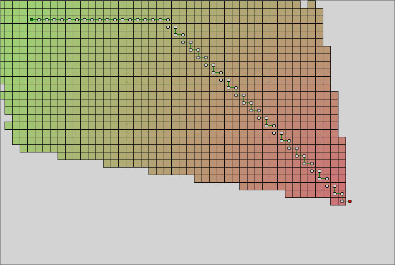 The so-called Manhattan method is used fairly often — it computes the minimum distance you’d have to travel along the coordinate axes to reach a given point:
h = D * (|x-fx| + |y-fy|)
x, y — the current coordinates, fx, fy — the coordinates of the path’s end point, D — the weight of a single step.
The main drawback of this method is the “staircase” look of the resulting path.
Diagonal Distance
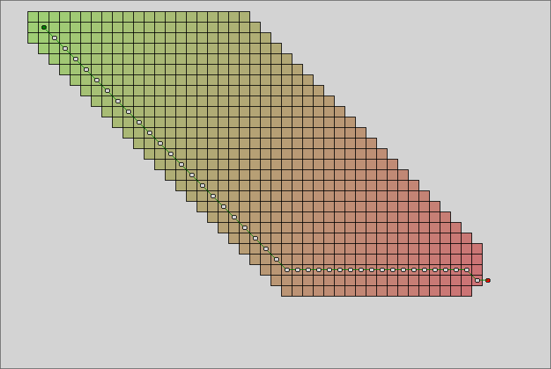 A more elaborate variant of the Manhattan function accounts for diagonal movement between cells. The formula takes into account which axis the path is longer along:
ax = |x-fx|
ay = |y-fy|
if ax > ay then
   h = ax * D * √2 + D * (ax - ay)
else
   h = ay * D * √2  + D * (ay - ax)
D — the weight of a step along the coordinate axes, D * √2 — the weight of a diagonal step. This function is perfectly balanced, and despite exploring a large number of points, it produces an optimal path in a reasonable amount of time.
Euclidean Distance
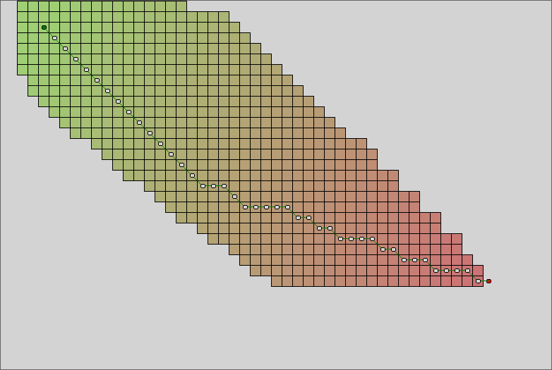 Another approach is to use the actual straight-line distance to the end point. In this case the function isn’t perfectly balanced, because the distance g is computed accounting for movement in 8 directions, while the distance from a point to the goal is measured as the crow flies. A* will still produce an optimal path, but it will check a somewhat larger number of points:
         _________________
h = D * √(x-fx)² + (y-fy)²
Squared Euclidean Distance
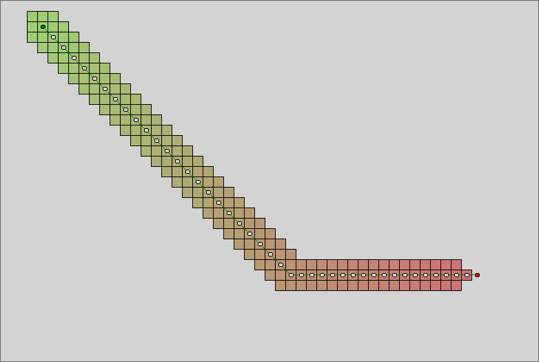 This method gets branded as pseudoscientific and wrong in a lot of sources. The problem is that the function’s value ends up noticeably larger than the traveled distance g, so instead of finding the optimal path the algorithm ends up sort of “gravitating” toward the end point. The formula looks like this:
h = D * ((x-fx)² + (y-fy)²)
That’s exactly the mistake I made in my own implementation — I forgot to add the square root — but as a result the number of points checked came out several times lower than with the other functions!
Things get more complicated once obstacles are added. The quadratic function: 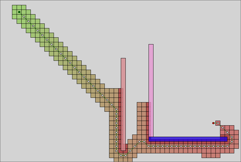
The diagonal function: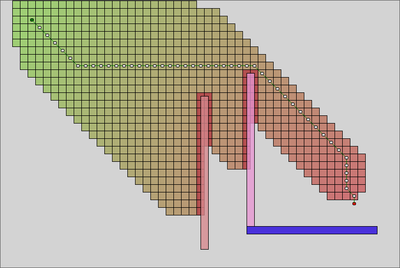
In the second case the path is “more correct,” but a lot of extra points got checked along the way. To be honest, the first variant isn’t really A* at all — it doesn’t return the most optimal path, just the first one it finds. That suited me fine — in real life characters rarely move perfectly anyway, so for AI purposes this kind of algorithm works well enough. The only thing left unsolved was the very problem that got me digging into heuristics in the first place — the path’s excessive “geometric” look.
The Compass Algorithm
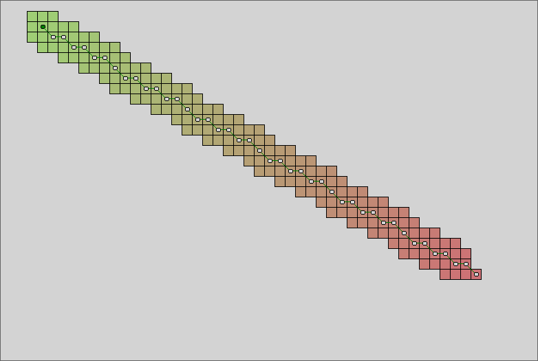 I couldn’t come up with a proper name for this algorithm. Its author (Amit Patel) described it like this:
A different way to break ties is to prefer paths that are along the straight line from the starting point to the goal
The idea is similar to navigating by a compass — once you have a heading, after going around an obstacle you should keep moving in the same direction as before. The base heuristic formula stays the same, but a small offset gets added to it:
cross = |(x-fx)*(y-sy) - (y-fy)*(x-sx)|
h = h + cross * k
sx, sy — the coordinates of the starting point, k — the offset coefficient (0.001 in the algorithm author’s version), cross — the magnitude of the cross product between the movement vector for the current point and the starting point.
For open spaces this function works very well, but going around obstacles introduces some error, which can be controlled by adjusting k. I never did find a value for this coefficient where the path stays optimal without a “backtracking” artifact showing up: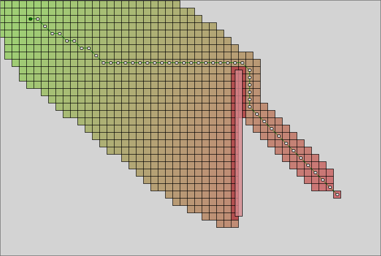
The “Homing” Algorithm
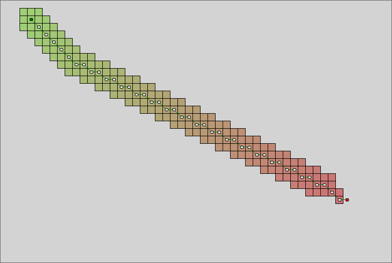 Out of all these experiments I came up with my own algorithm, similar to the “compass” one, but instead of pulling toward the line between the start and end points, it pulls toward the line between the previously visited point and the end point:
cross = |(x-fx)*(y-py) - (y-fy)*(x-px)|
h = h + cross * k
px, py — the coordinates of the previously visited point. This approach doesn’t give a perfect picture for movement without obstacles, but with a coefficient of k = 0.5, obstacle avoidance looks quite correct: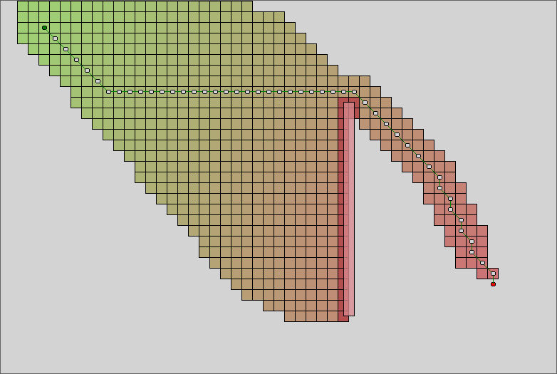
This kind of heuristic produces an optimal path and solves most of A*’s problems, especially movement across open terrain. In my view, though, these advantages never outweighed the computation speed of the “wrong” quadratic function. For example, with the same obstacle and no extra tweaks, it handles things like this: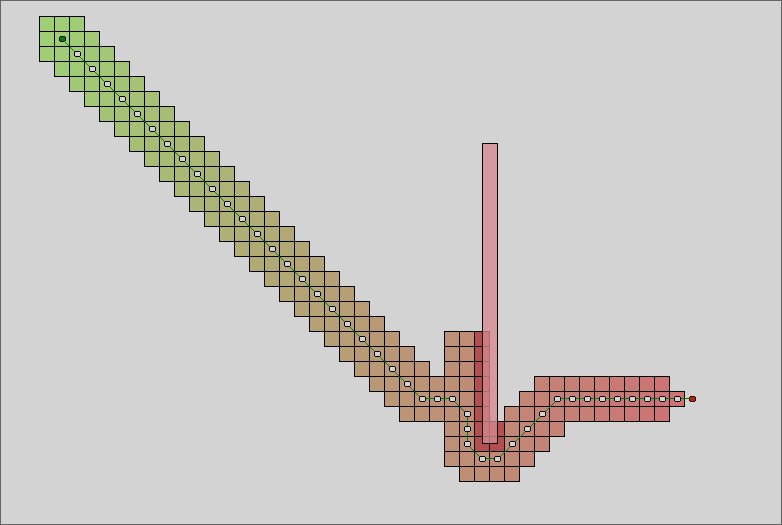
So I decided to keep exploring the direction of a shifted balance and leave a choice of working modes — “accurate” and “fast.”
The “Greedy” Algorithm
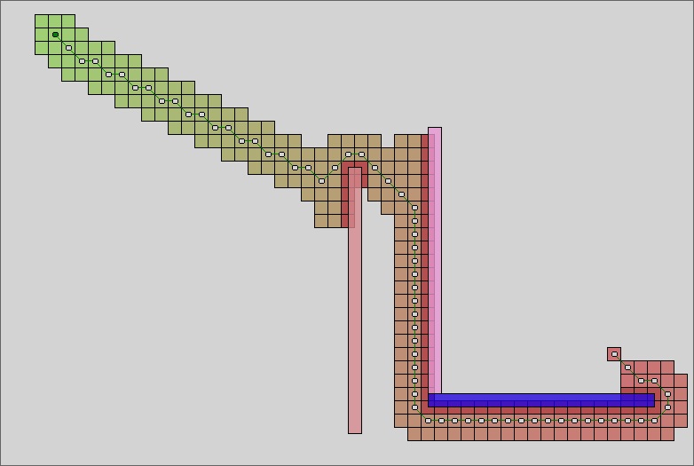 Further searching led to a function that flatly ignores the balance between g and h. This turned the algorithm from A* into what’s essentially Greedy Search, which, oddly enough, runs very fast and looks perfectly natural for AI purposes.
The formula is:
ax = |x-fx|
ay = |y-fy|
if ax > ay then
   h = ax * D * n
else
   h = ay * D * n
cross = |(x-fx)*(y-sy) - (y-fy)*(x-sx)|
h = h + cross * k
n — the weight factor, k — the “homing” coefficient.
In the illustration above, the coefficients are 100 and 1 respectively.
Conclusion
This isn’t meant to push any particular agenda. For our own needs I decided to use both plain A* and the “greedy” algorithm side by side, but in a lot of situations you need maximum accuracy and greedy algorithms just don’t apply. Either way, I hope this article is useful to anyone who wants to understand how A* works and what its heuristic function can do.
P.S. Finally, a few “live” examples of the greedy algorithm at work.
Medium density. The calculation took 228ms, 2689 points, 5289 visibility checks: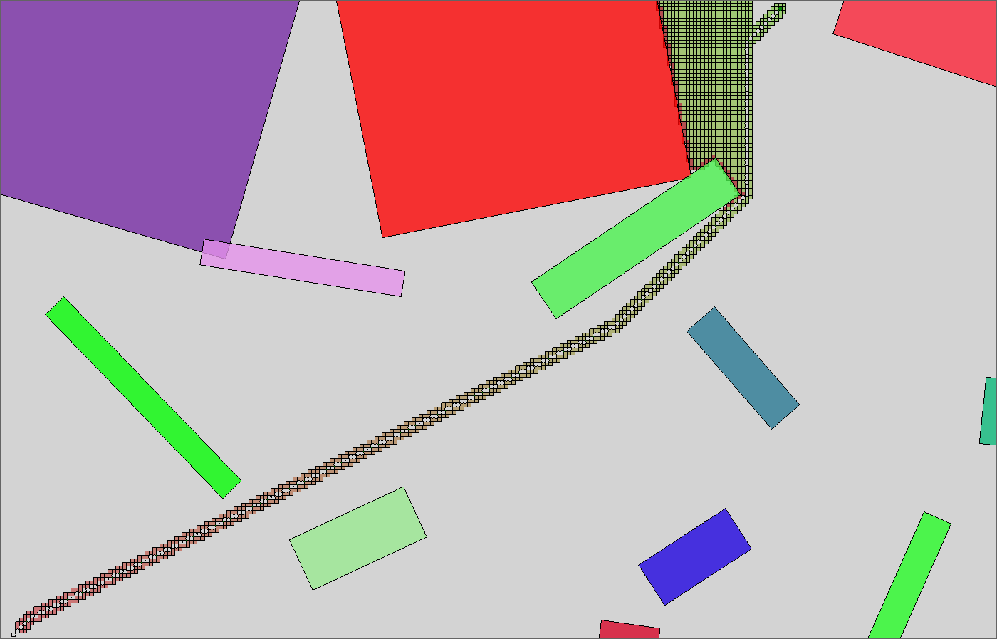
High density. The calculation took 274ms, 2177 points, 4110 visibility checks: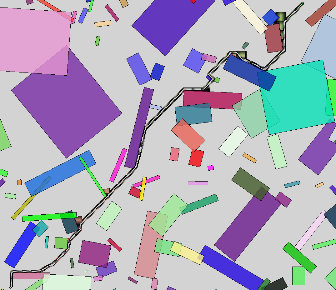
Originally published 2010-12-23.