
How I Measured the Evolution of Sysadmins into Programmers

Recently my acquaintance Karl (name changed) was interviewing for a DevOps position and asked me to check his solution. I read through the problem statement and decided it would make a decent test, so I expanded it a bit and wrote my own implementation, and also asked my colleague Alex to think up his own implementation. Once all three versions were ready, I put together two more comparison versions in C# and sat down to write this article. The task is fairly simple, and the candidates sit at various stages of the evolution from sysadmin to programmer, which is exactly what I wanted to measure.
Anyone interested in the messy details, non-objective tests, and subjective ratings, read on below the cut.
The task
By the terms of the problem, we have text logs of server CPU load and need to run certain queries against them.
As a result, for 1000 servers with 2 CPUs each, over one day you end up with a directory containing 1000 text logs, each with 2880 records in this format:
1414689783 192.168.1.10 0 87
1414689783 192.168.1.11 1 93
The fields in the file mean the following:
timestamp IP cpu_id usage
You need to write a CLI program that takes the name of the log directory as a parameter and lets you look up the load of a specific processor over a time range.
The program may take an unlimited amount of time to initialize, but the execution time of each individual query must be under one second.
The following query commands need to be supported:
1. The QUERY command — summary statistics for a server over a time range
Syntax: IP cpu_id time_start time_end
*Time is given as YYYY-MM-DD HH:MM
Example:
>QUERY 192.168.1.10 1 2014-10-31 00:00 2014-10-31 00:05
(2014-10-31 00:00, 90%), (2014-10-31 00:01, 89%), (2014-10-31 00:02, 87%), (2014-10-31 00:03, 94%), (2014-10-31 00:04, 88%)
2. The LOAD command — average load of the selected processor for the selected server
Syntax: IP cpu_id time_start time_end
Example:
>LOAD 192.168.1.10 1 2014-10-31 00:00 2014-10-31 00:05
88%
3. The STAT command — statistics for all processors on the selected server
Syntax: IP time_start time_end
Example:
>STAT 192.168.1.10 2014-10-31 00:00 2014-10-31 00:05
0: 23%
1: 88%
Any programming language or third-party utilities may be used.
P.S. The original assignment implied this would be an interactive program that accepts commands from the console after loading. That’s not mandatory, and the program can be split into separate parts for loading and for running queries. I.e. a version with several scripts — init.sh, query.sh, load.sh, etc. — is acceptable too.
Overall, the task is fairly transparent and practically invites the use of a database, so it’s no surprise that all three solutions use SQLite. I also made auxiliary C# versions for comparing speed, and they work differently.
Evaluation
For the finished solutions I scored two factors with a 40/60% weighting: speed and code quality. The scoring method for both factors is described a bit further below, but neither factor really speaks to the overall question or shows the degree of “sysadmin-ness” or “programmer-ness,” so on top of the raw speed/quality scores I also derived a separate subjective scale: “sysadmin solution,” “programmer solution,” “universal solution.” This is in no way a competition or a comparison of language speeds, but rather an evaluation of approaches to programming.
Speed scoring
Per the assignment, a query needs to run in under a second, but there’s no mention of hardware, core count, or the test machine’s architecture at all. In my view that suggests the test should run an order of magnitude or two faster, so that on reasonable hardware it always stays comfortably within budget. This should also point toward the idea of scalability — the task gives an example with 2,880,000 records for a single day, but in real conditions there could be noticeably more (more servers and cores), and the query range might cover not days but months or years. So an ideal solution shouldn’t show any dependency on data volume and shouldn’t consume limited resources without bound. In that light, uncontrolled memory use (in-memory tables or storing everything in arrays in memory) is a minus, not a plus, because a year’s worth of data for 10,000 machines with 8 processors each works out, roughly, to 42,048,000,000 records, at least 10 bytes each, i.e. ~420GiB of data. Unfortunately I wasn’t able to test at that scale given the hardware I had available.
Speed was measured with the unix time command (the user value), and for interactive solutions, with internal timers inside the program.
Quality scoring
By quality I mainly mean versatility — versatility of use, of maintenance, of further development. There’s not much point in code that only works within strictly defined bounds and can’t step outside them, handle more data, or be adapted to other situations, and so on. For example, x86 Assembler code could be extremely fast but completely inflexible, and even a simple change like switching to IPv6 addresses could be very painful for it. First and foremost I evaluated handling of input parameters here: edge cases, queries that return zero results, invalid requests. Second came the programming language, code style, and the amount and quality of comments.
Subjective scoring
It’s hard to say exactly which parameter determines how far an admin has evolved toward being a programmer. Personally, I split it along these lines: an admin works with tools, a programmer creates them. It’s roughly the difference between a professional race driver and an auto mechanic — a mechanic often drives quite well and knows the car inside out, but the driver feels everything the car is capable of, and then some. A good admin knows how fast a database runs, understands what horizontal and vertical scaling mean, and uses indexes every day. A programmer might write their own database, use nested trees for it, convert all the data into a custom format and lay it out on disk in some clever way for fast access.
If Karl had written brute-force scanning of the data, citing its supposedly superior performance, especially combined with hashing or fast search, that would have suggested he’d already become a programmer. But it probably wouldn’t have gotten him the DevOps job.
The programs
In total I had 5 programs — three take part in the comparison, and two were written later, purely to check a couple of ideas, in C#. For convenience I’ll refer to the programs by their authors’ names.
Karl
Code on github
Language: Python 2.7
Dependencies: none
Interactive: yes
DB: SQLite, in-memory table
Alex
Code on github
Language: Python 2.7
Dependencies: progress, readline
Interactive: yes
DB: SQLite, in-memory table
Nomad1
Code on github
Language: Bash
Dependencies: none
Interactive: no
DB: SQLite
Notable feature: external .db file to work with
Nomad2
Code on github
Language: C#
Dependencies: mono
Interactive: yes
DB: none
Notable feature: hash table keyed by IP address
Nomad3
Code on github
Language: C#
Dependencies: mono
Interactive: no
DB: none
Notable feature: specially pre-prepared data
Testing
For testing I wrote a log generator, first in bash, then in C++. Three test data sets were created:
- data_norm — 1000 logs with 2 CPUs each, one day (~80Mb of logs)
- data_wide — 1000 logs with 2 CPUs each, one month (~2.3Gb of logs)
- data_huge — 10000 logs with 4 CPUs each, 5 days (~10Gb of logs)
Queries were built along these lines:
- valid — a query within the range of valid values
- wide — a query wider than the valid range (spans the start or end of the range)
- invalid — a query for data that doesn’t exist
Every test was run 4 times; the first value was discarded and the rest were averaged (to rule out JIT compilation time, cache warm-up, and paging back in from swap). Testing was done on a work machine running Mac OS 10.13.2 with an i7 2.2 GHz CPU, 8GB RAM, and an SSD.
Unfortunately, the QUERY test results aren’t very representative for half the programs, since printing to screen is often several times slower than the query itself. In Nomad1’s case, output can take hundreds of milliseconds due to very slow formatting in Bash, while the query itself runs in milliseconds. Karl’s program actually has a measurement bug: it times only the internal QUERY execution, without the screen output. To my mind, “command execution time” is the time between entering the command and getting the result, so I had to apply the penalties described below to this program.
Notably, Karl and Alex, without any coordination, both wrote their programs in python 2.7, using SQLite, in interactive mode (load the data first, then accept commands). Nomad1’s program is written in plain bash as a set of CLI scripts and also uses SQLite.
Nomad2 and Nomad3 are interesting for their shared approach: in Nomad2’s case, all the data is loaded into memory into a hash table keyed by IP. In Nomad3’s case, the filename is treated, by convention, as the IP address, and on lookup the program simply reads the file into memory and works by brute-force scan from there. Both of these tests only make sense for comparing speed and don’t take part in the quality scoring. On top of everything else, they’re written in C#, which on Unix comes in the form of mono and has a whole bunch of quirks. For example, mono32 and mono64 results differ by multiples for the same code, and on Windows with .Net everything runs even faster still.
Speed results
I’ll tuck the actual query commands under a spoiler so as not to clutter up the article. In the result tables, each cell has three lines — these are the execution times for the QUERY, LOAD, and STAT commands, in seconds.
QUERY 10.0.2.23 1 2014-10-31 09:00 2014-10-31 12:00
LOAD 10.0.2.254 0 2014-10-31 13:10 2014-10-31 20:38
STAT 10.0.1.1 2014-10-31 04:21 2014-10-31 08:51
data_norm/wide:
QUERY 10.0.1.11 0 2014-10-01 09:00 2014-10-31 07:21
LOAD 10.0.2.254 1 2014-10-31 15:55 2014-11-04 10:00
STAT 10.0.1.100 2014-10-31 14:21 2015-01-01 01:01
data_norm/invalid
QUERY 10.0.2.23 1 2015-10-31 09:00 2015-10-31 12:00
LOAD 10.0.2.254 0 2015-10-31 13:10 2015-10-31 20:38
STAT 10.0.1.1 2015-10-31 04:21 2015-10-31 08:51
data_wide/valid:
QUERY 10.0.2.33 0 2014-10-30 09:00 2014-10-31 02:00
LOAD 10.0.0.125 1 2014-10-02 14:04 2014-10-04 20:38
STAT 10.0.1.10 2014-10-07 00:00 2014-10-17 23:59
data_wide/wide:
QUERY 10.0.1.11 1 2014-07-30 09:00 2014-10-01 07:21
LOAD 10.0.0.137 0 2014-10-20 04:12 2015-02-01 00:00
STAT 10.0.3.3 2014-10-20 04:12 2015-02-01 00:00
data_wide/invalid
QUERY 10.0.0.123 1 2015-10-31 09:00 2015-10-31 12:00
LOAD 10.0.0.154 0 2015-10-31 13:10 2015-10-31 20:38
STAT 10.0.0.1 2015-10-31 04:21 2015-10-31 08:51
data_huge/valid:
QUERY 10.0.2.33 0 2014-10-30 09:00 2014-10-31 02:00
LOAD 10.0.0.125 1 2014-10-28 14:04 2014-10-30 20:38
STAT 10.0.1.10 2014-10-28 00:00 2014-10-30 23:59
data_huge/wide:
QUERY 10.0.5.72 0 2014-10-31 09:00 2015-11-03 12:11
LOAD 10.0.0.137 0 2014-10-20 04:12 2015-02-01 00:00
STAT 10.0.3.3 2014-10-20 04:12 2015-02-01 00:00
data_huge/invalid
QUERY 10.0.1.11 1 2014-07-30 09:00 2014-10-01 07:21
LOAD 10.0.0.154 0 2015-10-31 13:10 2015-10-31 20:38
STAT 10.0.0.1 2015-10-31 04:21 2015-10-31 08:51
135 tests were run (27 per program), and their execution times are given in the table below:
| Test | Karl | Alex | Nomad1 | Nomad2 | Nomad3 |
|---|---|---|---|---|---|
| data_norm/valid | 0.008800 0.000440 0.000420 |
0.215300 0.211700 0.217800 |
0.256200 0.007300 0.008300 |
0.002160 0.000130 0.000140 |
0.050200 0.050300 0.052600 |
| data_norm/wide | 0.002640 0.000330 0.000630 |
0.218000 0.212000 0.215000 |
0.716000 0.008000 0.008600 |
0.005000 0.000150 0.000320 |
0.050200 0.005200 0.005500 |
| data_norm/invalid | 0.000063 0.000073 0.000065 |
0.214200 0.209100 0.206300 |
0.007600 0.008300 0.008100 |
0.000008 0.000026 0.000034 |
0.048000 0.053000 0.050000 |
| data_wide/valid | 0.007300 0.005500 0.002300 |
6.237600 6.146500 6.151000 |
1.446000 0.036000 0.069000 |
0.017186 0.001099 0.005665 |
0.167000 0.088000 0.126000 |
| data_wide/wide | 0.006800 0.002100 0.024200 |
6.176600 6.157900 6.326100 |
0.570000 0.039000 0.070000 |
0.008363 0.005818 0.005592 |
0.071000 0.160000 0.159000 |
| data_wide/invalid | 0.000085 0.000110 0.000150 |
6.288100 6.152100 6.130400 |
0.044000 0.040000 0.062000 |
0.000013 0.000040 0.000013 |
0.155000 0.156000 0.164000 |
| data_huge/valid | 0.009107 0.007655 0.012858 |
155.9738 146.5377 140.1752 |
1.401000 0.013300 0.026000 |
0.036806 0.003798 0.003751 |
0.069000 0.066000 0.072000 |
| data_huge/wide | 0.009418 0.013718 0.014266 |
157.1896 148.5435 147.9525 |
1.078000 0.011700 0.026000 |
0.018393 0.000805 0.003329 |
0.072000 0.081000 0.077000 |
| data_huge/invalid | 0.000070 0.000095 0.000081 |
144.7307 158.0090 165.6820 |
0.012000 0.013000 0.023000 |
0.000012 0.000031 0.000013 |
0.054000 0.071000 0.081000 |
I scored speed mathematically: for each query and each data set I took the order of magnitude (base-10 log of the time in microseconds), then used it as a divisor against the order of magnitude of the fastest solution. That way the fastest solution gets a coefficient of 1.0, one order of magnitude slower gets 0.5, and so on. The result for each program is averaged and multiplied by 40.
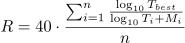
For Karl’s program I unfortunately had to apply a penalty coefficient, since it didn’t time the whole QUERY command, only the internal SQL query. I added one order of magnitude (M) to all non-empty QUERY results, which knocked about 2 points total off Karl’s score.
The full results table can be seen here.
Results:
Karl: 31/40 (33 without penalty)
Alex: 15/40
Nomad1: 22/40
Nomad2: 39/40
Nomad3: 21/40
Quality results
The speed tests turned up a number of interesting bugs and pitfalls. I’m tucking them under a spoiler in case you get the urge to write your own version of this program and are sure you won’t make the same mistakes as everyone else. Nomad2 and Nomad3 aren’t examined or scored here.
2. Indexes. Alex forgot about indexes entirely. Karl created an index on every field — IP + Timestamp + CPU. That’s only justified in fairly rare cases of looking up an exact Timestamp, but per the assignment we always query by IP + CPU and a Timestamp range. Not critical if the database size stays reasonably modest, but for the _wide and _huge variants this led to huge memory losses for minimal speed gain. Karl’s program on the _huge data kept crashing with “Killed: 9” from memory and swap exhaustion.
3. Including range boundaries in calculations. Nomad1 forgot about this, and due to some quirk in timestamp conversion in bash, its query sometimes doesn’t include the lower boundary (there’s a fixed version on github, but it wasn’t part of the tests).
4. Using an :memory: table with an unknown data volume.
This is an architectural mistake made by both Karl and Alex — they used an in-memory table without asking themselves about the consequences or the data volumes involved. As a result, their programs are very sensitive to data size and available memory, which already shows up in the data_huge test. In real-world conditions programs like this either wouldn’t work at all, or would work with problems. The ideal solution should estimate the volume of data being read and pick a database type accordingly.
5. Validating input data and errors. Everyone dropped the ball here — queries to the database aren’t checked for valid dates, addresses, SQL injection, and so on. For an invalid LOAD query, Alex’s program throws a divide-by-zero error, Karl’s prints “No data,” and Nomad1’s has no exception handling at all, and the SQLite error output in a STAT query gets mangled by splitting the string on the | character. None of the programs accepts an IP address in the form 010.00.020.003. All of them crashed on some invalid queries, but since testing required 540+ command executions, I didn’t have the stamina to collect and analyze every example.
6. Rounding results for LOAD and STAT. Karl didn’t round anything and printed a number with a decimal point, which isn’t fatal but doesn’t match the assignment’s requirements. Alex cast the number to INT, dropping the fractional part entirely.
All three programs are written in modern, readable programming languages (no VBScript or Brainfuck spotted). The bash code is somewhat less readable than the Python versions, but noticeably shorter. Alex’s code uses the third-party readline and progress libraries, has its own class for Tab autocomplete, separate functions for help text, date handling, support for reloading data, and error handling, though the database isn’t closed on exit. Karl’s code uses a class inherited from Cmd, has exception handling, closes the database on exit, and catches Ctrl-C. Unfortunately nobody left comments (with a couple of minor exceptions).
Alex takes an interesting, more programmer-like approach — he runs the same query for all three commands, then computes the data for STAT/LOAD in code, without relying on AVG and GROUP BY. This significantly cuts down the amount of code, while the execution speed ends up roughly the same as offloading the work to the database.
Taking these points and a couple of additional quality factors into account, I scored the programs as follows:
Karl: 35/60
Alex: 40/60
Nomad1: 30/60
Conclusions
Total scores:
Karl: 66/100
Alex: 55/100
Nomad: 52/100
On both points and speed, Karl’s solution came out on top overall, since Alex’s solution isn’t competitive on speed due to the lack of indexes. Interestingly, as soon as I told Alex about the low speed, he said that indexes could be added at line 82, that he’d planned and thought it through, but decided to leave it “for later.” Unfortunately, that was already after submissions closed and the code was frozen, so that change couldn’t be made.
Nomad2 and Nomad3 scored 39/40 and 21/40 on speed respectively. Unsurprising that working with a hash table turned out faster than a database, even at the cost of much higher memory use. Working directly with the filesystem wasn’t especially fast, but you have to keep in mind that this approach has almost no initialization time, minimal memory pressure, and can, in principle, be used with any volume of pre-prepared data.
Karl’s variant, due to its “wide” index, consumed more memory than anything else and started failing already at a data size of 6GB. Any variant using an :memory: table or a hash table won’t be able to handle 10GB and up, while the file-based database solution is barely slower and scales far better. Unfortunately, printing output through bash sealed that program’s fate on speed.
Building things as interactive applications gives a substantial speed boost — you can clearly see with Nomad1 and Nomad3 that even on empty queries, about 10ms for bash and 50ms for C# goes purely into startup.
Subjective evaluation
Now for a bit of subjective rambling. Anyone easily annoyed can skip this part; as a reminder, everything written here is purely my own opinion and probably won’t match yours.
All three participants used SQLite and didn’t try to reinvent the wheel. That’s undoubtedly a plus, but it also clearly shows that all three solutions are far from pure programming. They solve the task, and reasonably fast at that, but without any attempt to build a custom in-memory database with fast indexing (as in the Nomad2 variant) or querying without upfront loading (as in the Nomad3 variant). Alex’s approach of using a single query and then computing LOAD/STAT in code is a bit closer to a programmer’s solution. I also didn’t see other “hallmarks of a programmer” in the code, such as logging, comments, or custom data structures (an IPv4 address is, after all, a 32-bit number, and CPU and LOAD are single-byte values!). Overall, the authors didn’t really stop to think about data storage and, broadly speaking, just moved the text files over into SQLite’s binary format.
So in my view, on the subjective scales, the solutions rank like this:
Most “sysadmin” solution:
1. Nomad1 — both the .import command and piping data straight into the sqlite console client instead of using a connector/cursor
2. Karl — working with indexes, SQL queries for every operation, GROUP BY, ORDER BY
3. Alex
Most “programmer” solution (the “built a new tool” perk):
1. Alex — good structure, working with an array of data during selection, third-party libraries
2. Karl — code with exception handling, data cleanup
3. Nomad1
Most “universal” solution:
1. Nomad1 — commands are just added as separate query files against a ready-made DB, following the existing pattern; the program doesn’t depend on data volume or memory
2. Alex — a single query yields an array of data that the code then processes; there’s already code at the top of the file for working with a file-based DB
3. Karl
All the program code, including the generator, is available on GitHub
It also includes the commands used for generating the data sets.
If anyone wants to test themselves on a similar problem, be my guest.
P.S.: Going by the test results, Nomad1 — a programmer with 20 years of experience — scored lower on this task than the DevOps candidate and the junior developer. On the other hand, he’s also the author of this article, and it would be, ahem, rather improper to award himself higher marks 🙂
P.P.S.: Writing this article and running the measurements took three working days, more than all the participants combined spent writing and debugging their code. The author’s productivity as a writer is, unambiguously, unsatisfactory.
Originally published on Habr, 2018-05-27.